Visualize Results in the Pipelines UI
Old Version
This page is about Kubeflow Pipelines V1, please see the V2 documentation for the latest information.
Note, while the V2 backend is able to run pipelines submitted by the V1 SDK, we strongly recommend migrating to the V2 SDK.
For reference, the final release of the V1 SDK was kfp==1.8.22, and its reference documentation is available here.
This page shows you how to use the Kubeflow Pipelines UI to visualize output from a Kubeflow Pipelines component.
Introduction
The Kubeflow Pipelines UI offers built-in support for several types of visualizations, which you can use to provide rich performance evaluation and comparison data. Follow the instructions below to write visualization output data to the file system. You can do this at any point during the pipeline execution.
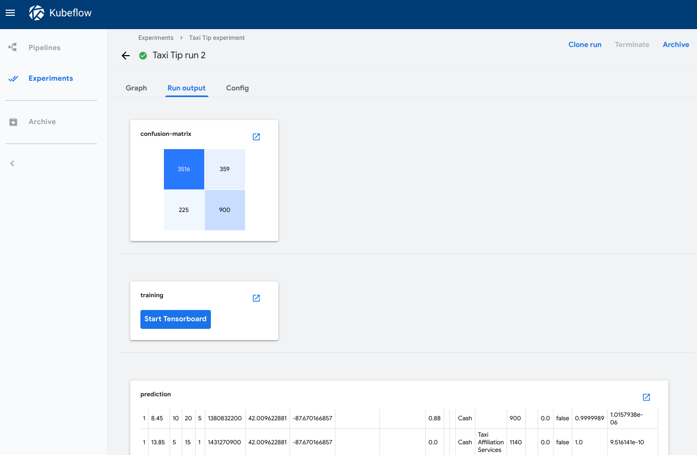
You can view the output visualizations in the following places on the Kubeflow Pipelines UI:
The Run output tab shows the visualizations for all pipeline steps in the selected run. To open the tab in the Kubeflow Pipelines UI:
- Click Experiments to see your current pipeline experiments.
- Click the experiment name of the experiment that you want to view.
- Click the run name of the run that you want to view.
- Click the Run output tab.
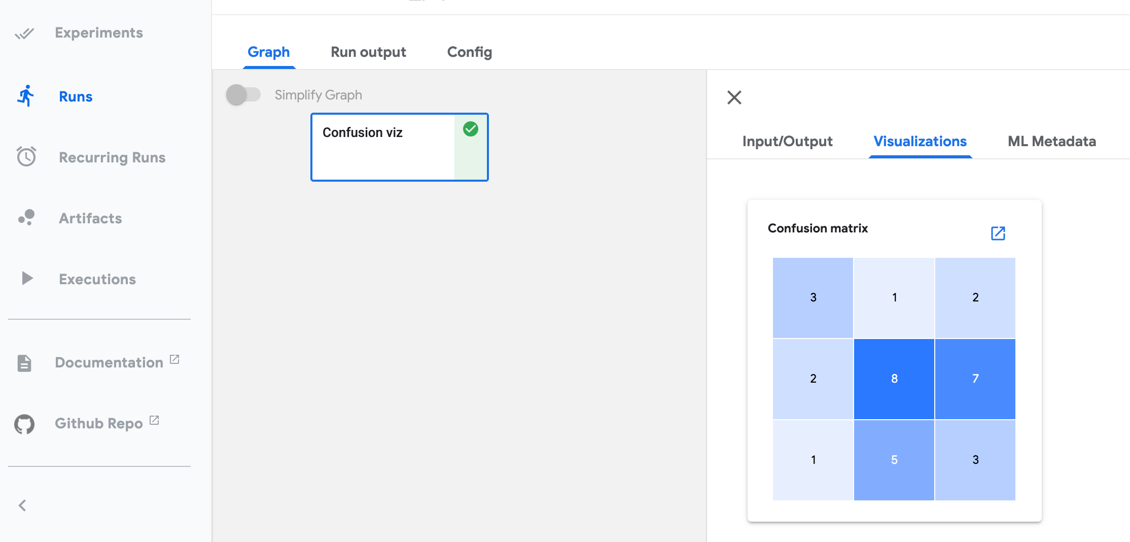
The Visualizations tab shows the visualization for the selected pipeline step. To open the tab in the Kubeflow Pipelines UI:
- Click Experiments to see your current pipeline experiments.
- Click the experiment name of the experiment that you want to view.
- Click the run name of the run that you want to view.
- On the Graph tab, click the step representing the pipeline component that you want to view. The step details slide into view, showing the Visualizations tab.
All screenshots and code snippets on this page come from a sample pipeline that you can run directly from the Kubeflow Pipelines UI. See the sample description and links below.
v2 SDK: Use SDK visualization APIs
For KFP SDK v2 and v2 compatible mode, you can use convenient SDK APIs and system artifact types for metrics visualization. Currently KFP supports ROC Curve, Confusion Matrix and Scalar Metrics formats. Full pipeline example of all metrics visualizations can be found in metrics_visualization_v2.py.
Requirements
- Use Kubeflow Pipelines v1.7.0 or above: upgrade Kubeflow Pipelines.
- Use
kfp.dsl.PipelineExecutionMode.V2_COMPATIBLEmode when you compile and run your pipelines. - Make sure to use the latest environment kustomize manifest pipelines/manifests/kustomize/env/dev/kustomization.yaml.
For a usage guide of each metric visualization output, refer to sections below:
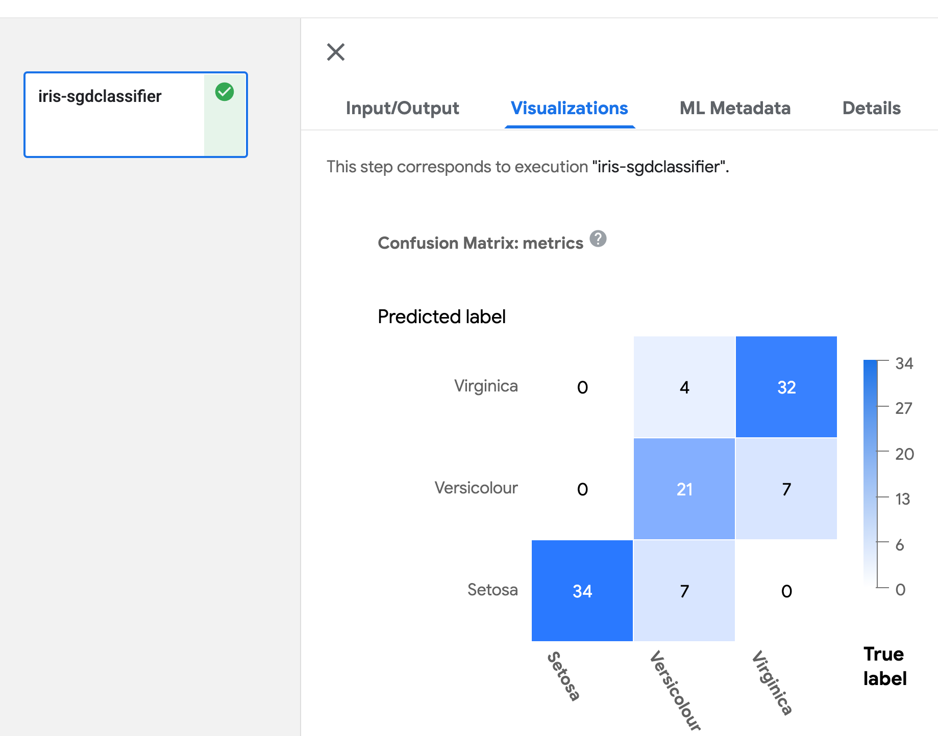
Confusion Matrix
Define Output[ClassificationMetrics] argument in your component function, then
output Confusion Matrix data using API
log_confusion_matrix(self, categories: List[str], matrix: List[List[int]]). categories
provides a list of names for each label, matrix provides prediction performance for corresponding
label. There are multiple APIs you can use for logging Confusion Matrix. Refer to
artifact_types.py for detail.
Refer to example below for logging Confusion Matrix:
@component(
    packages_to_install=['sklearn'],
    base_image='python:3.9'
)
def iris_sgdclassifier(test_samples_fraction: float, metrics: Output[ClassificationMetrics]):
    from sklearn import datasets, model_selection
    from sklearn.linear_model import SGDClassifier
    from sklearn.metrics import confusion_matrix

    iris_dataset = datasets.load_iris()
    train_x, test_x, train_y, test_y = model_selection.train_test_split(
        iris_dataset['data'], iris_dataset['target'], test_size=test_samples_fraction)


    classifier = SGDClassifier()
    classifier.fit(train_x, train_y)
    predictions = model_selection.cross_val_predict(classifier, train_x, train_y, cv=3)
    metrics.log_confusion_matrix(
        ['Setosa', 'Versicolour', 'Virginica'],
        confusion_matrix(train_y, predictions).tolist() # .tolist() to convert np array to list.
    )

@dsl.pipeline(
    name='metrics-visualization-pipeline')
def metrics_visualization_pipeline():
    iris_sgdclassifier_op = iris_sgdclassifier(test_samples_fraction=0.3)
Visualization of Confusion Matrix is as below:
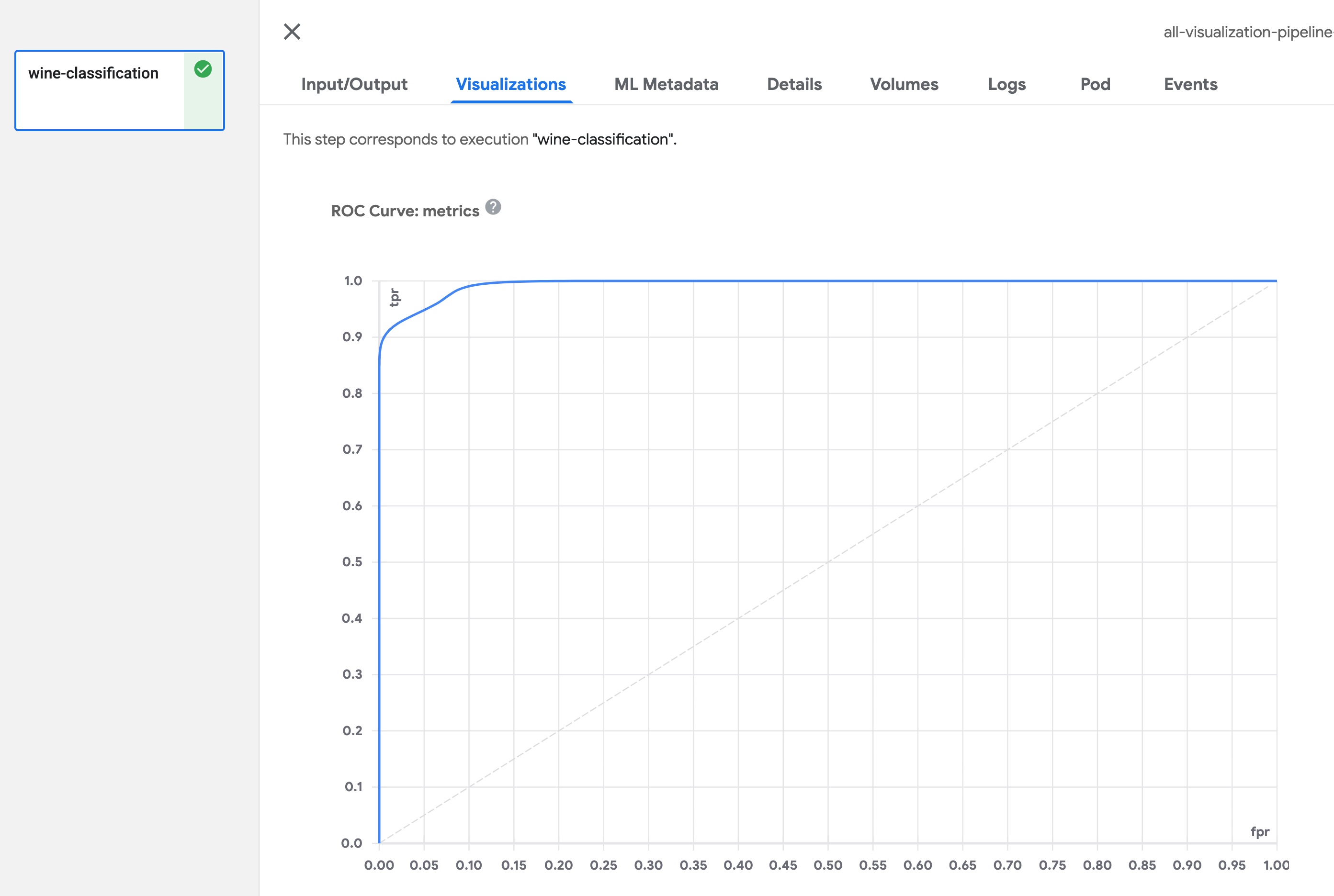
ROC Curve
Define Output[ClassificationMetrics] argument in your component function, then
output ROC Curve data using API
log_roc_curve(self, fpr: List[float], tpr: List[float], threshold: List[float]).
fpr defines a list of False Positive Rate values, tpr defines a list of
True Positive Rate values, threshold indicates the level of sensitivity and specificity
of this probability curve. There are multiple APIs you can use for logging ROC Curve. Refer to
artifact_types.py for detail.
@component(
    packages_to_install=['sklearn'],
    base_image='python:3.9',
)
def wine_classification(metrics: Output[ClassificationMetrics]):
    from sklearn.ensemble import RandomForestClassifier
    from sklearn.metrics import roc_curve
    from sklearn.datasets import load_wine
    from sklearn.model_selection import train_test_split, cross_val_predict

    X, y = load_wine(return_X_y=True)
    # Binary classification problem for label 1.
    y = y == 1

    X_train, X_test, y_train, y_test = train_test_split(X, y, random_state=42)
    rfc = RandomForestClassifier(n_estimators=10, random_state=42)
    rfc.fit(X_train, y_train)
    y_scores = cross_val_predict(rfc, X_train, y_train, cv=3, method='predict_proba')
    y_predict = cross_val_predict(rfc, X_train, y_train, cv=3, method='predict')
    fpr, tpr, thresholds = roc_curve(y_true=y_train, y_score=y_scores[:,1], pos_label=True)
    metrics.log_roc_curve(fpr, tpr, thresholds)

@dsl.pipeline(
    name='metrics-visualization-pipeline')
def metrics_visualization_pipeline():
    wine_classification_op = wine_classification()
Visualization of ROC Curve is as below:
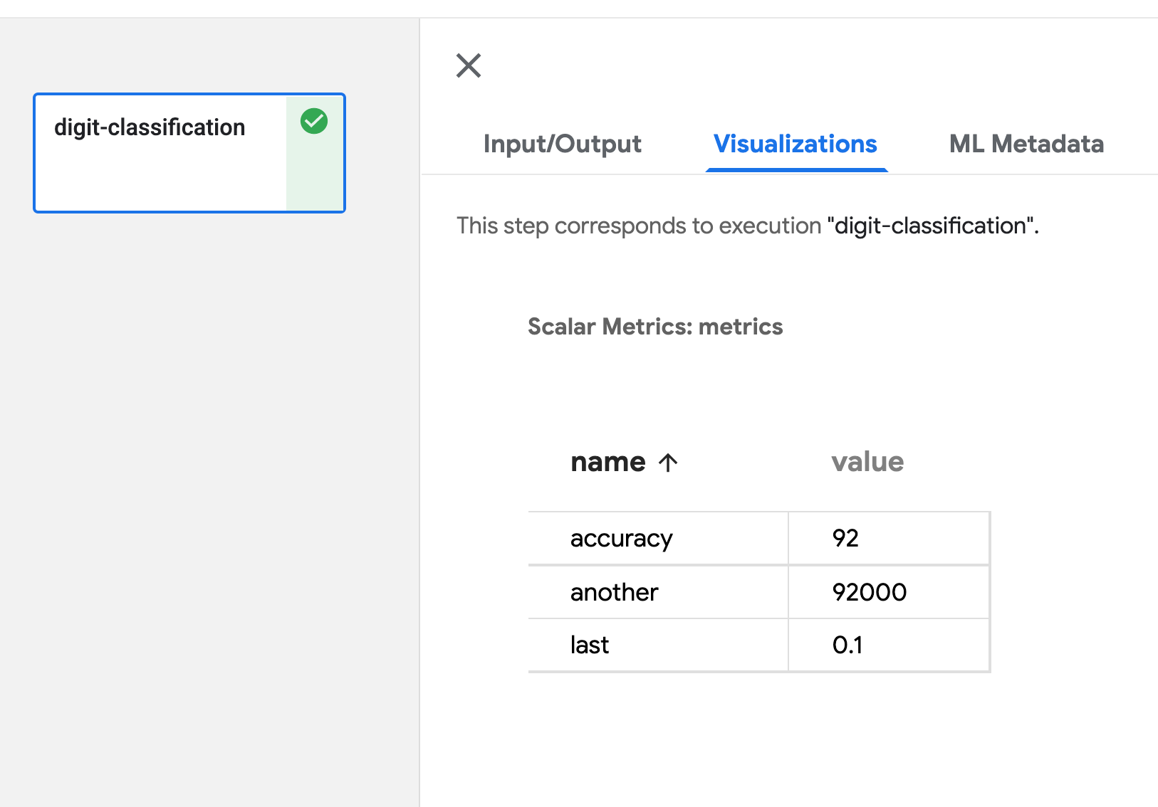
Scalar Metrics
Define Output[Metrics] argument in your component function, then
output Scalar data using API log_metric(self, metric: str, value: float).
You can define any amount of metric by calling this API multiple times.
metric defines the name of metric, value is the value of this metric. Refer to
artifacts_types.py
for detail.
@component(
    packages_to_install=['sklearn'],
    base_image='python:3.9',
)
def digit_classification(metrics: Output[Metrics]):
    from sklearn import model_selection
    from sklearn.linear_model import LogisticRegression
    from sklearn import datasets
    from sklearn.metrics import accuracy_score

    # Load digits dataset
    iris = datasets.load_iris()

    # # Create feature matrix
    X = iris.data

    # Create target vector
    y = iris.target

    #test size
    test_size = 0.33

    seed = 7
    #cross-validation settings
    kfold = model_selection.KFold(n_splits=10, random_state=seed, shuffle=True)

    #Model instance
    model = LogisticRegression()
    scoring = 'accuracy'
    results = model_selection.cross_val_score(model, X, y, cv=kfold, scoring=scoring)

    #split data
    X_train, X_test, y_train, y_test = model_selection.train_test_split(X, y, test_size=test_size, random_state=seed)
    #fit model
    model.fit(X_train, y_train)

    #accuracy on test set
    result = model.score(X_test, y_test)
    metrics.log_metric('accuracy', (result*100.0))

@dsl.pipeline(
    name='metrics-visualization-pipeline')
def metrics_visualization_pipeline():
    digit_classification_op = digit_classification()
Visualization of Scalar Metrics is as below:
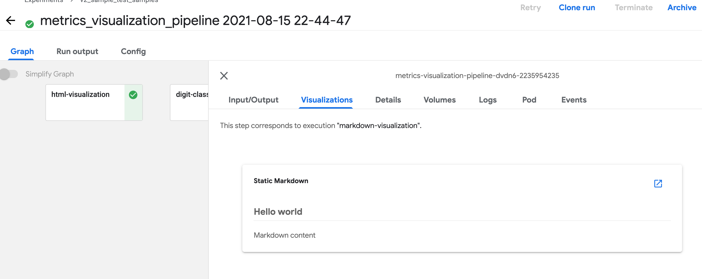
Markdown
Define Output[Markdown] argument in your component function, then
write Markdown file to path <artifact_argument_name>.path.
Refer to
artifact_types.py
for detail.
@component
def markdown_visualization(markdown_artifact: Output[Markdown]):
    markdown_content = '## Hello world \n\n Markdown content'
    with open(markdown_artifact.path, 'w') as f:
        f.write(markdown_content)
Single HTML file
You can specify an HTML file that your component creates, and the Kubeflow Pipelines UI renders that HTML in the output page. The HTML file must be self-contained, with no references to other files in the filesystem. The HTML file can contain absolute references to files on the web. Content running inside the HTML file is sandboxed in an iframe and cannot communicate with the Kubeflow Pipelines UI.
Define Output[HTML] argument in your component function, then
write HTML file to path <artifact_argument_name>.path.
Refer to
artifact_types.py
for detail.
@component
def html_visualization(html_artifact: Output[HTML]):
    html_content = '<!DOCTYPE html><html><body><h1>Hello world</h1></body></html>'
    with open(html_artifact.path, 'w') as f:
        f.write(html_content)
Source of v2 examples
The metric visualization in V2 or V2 compatible mode depends on SDK visualization APIs, refer to metrics_visualization_v2.py for a complete pipeline example. Follow instruction Compile and run your pipeline to compile in V2 compatible mode.
v1 SDK: Writing out metadata for the output viewers
For KFP v1, the pipeline component must write a JSON file specifying metadata
for the output viewer(s) that you want to use for visualizing the results. The
component must also export a file output artifact with an artifact name of
mlpipeline-ui-metadata, or else the Kubeflow Pipelines UI will not render
the visualization. In other words, the .outputs.artifacts setting for the
generated pipeline component should show:
- {name: mlpipeline-ui-metadata, path: /mlpipeline-ui-metadata.json}.
The JSON filepath does not matter, although /mlpipeline-ui-metadata.json
is used for consistency in the examples below.
The JSON specifies an array of outputs. Each outputs entry describes the
metadata for an output viewer. The JSON structure looks like this:
{
  "version": 1,
  "outputs": [
    {
      "type": "confusion_matrix",
      "format": "csv",
      "source": "my-dir/my-matrix.csv",
      "schema": [
        {"name": "target", "type": "CATEGORY"},
        {"name": "predicted", "type": "CATEGORY"},
        {"name": "count", "type": "NUMBER"},
      ],
      "labels": "vocab"
    },
    {
      ...
    }
  ]
}
If the component writes such a file to its container filesystem, the Kubeflow Pipelines system extracts the file, and the Kubeflow Pipelines UI uses the file to generate the specified viewer(s). The metadata specifies where to load the artifact data from. The Kubeflow Pipelines UI loads the data into memory and renders it. Note: You should keep this data at a volume that’s manageable by the UI, for example by running a sampling step before exporting the file as an artifact.
The table below shows the available metadata fields that you can specify in the
outputs array. Each outputs entry must have a type. Depending on value of
type, other fields may also be required as described in the list of output
viewers later on the page.
| Field name | Description |
|---|---|
format | The format of the artifact data. The default is csv.
Note: The only format currently available is
csv. |
header | A list of strings to be used as headers for the artifact data. For example, in a table these strings are used in the first row. |
labels | A list of strings to be used as labels for artifact columns or rows. |
predicted_col | Name of the predicted column. |
schema | A list of {type, name} objects that specify the schema
of the artifact data. |
source | The full path to the data. The available locations
include The path can contain wildcards ‘*’, in which case the Kubeflow Pipelines UI concatenates the data from the matching source files.
|
storage | (Optional) When Be aware, support for inline visualizations, other than markdown, was introduced in Kubeflow Pipelines 0.2.5. Before using these visualizations, [upgrade your Kubeflow Pipelines cluster](/docs/components/pipelines/legacy-v1/installation/upgrade//) to version 0.2.5 or higher. |
target_col | Name of the target column. |
type | Name of the viewer to be used to visualize the data. The list below shows the available types. |
Available output viewers
The sections below describe the available viewer types and the required metadata fields for each type.
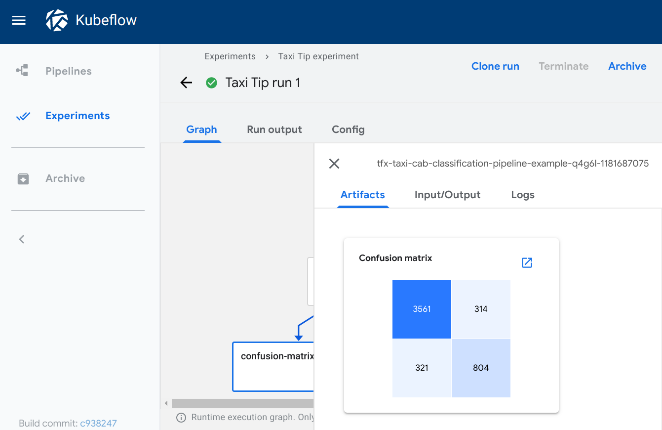
Confusion matrix
Type: confusion_matrix
Required metadata fields:
formatlabelsschemasource
Optional metadata fields:
storage
The confusion_matrix viewer plots a confusion matrix visualization of the data
from the given source path, using the schema to parse the data. The labels
provide the names of the classes to be plotted on the x and y axes.
Specify 'storage': 'inline' to embed raw content of the
confusion matrix CSV file as a string in source field directly.
Example:
def confusion_matrix_viz(mlpipeline_ui_metadata_path: kfp.components.OutputPath()):
  import json

  metadata = {
    'outputs' : [{
      'type': 'confusion_matrix',
      'format': 'csv',
      'schema': [
        {'name': 'target', 'type': 'CATEGORY'},
        {'name': 'predicted', 'type': 'CATEGORY'},
        {'name': 'count', 'type': 'NUMBER'},
      ],
      'source': <CONFUSION_MATRIX_CSV_FILE>,
      # Convert vocab to string because for bealean values we want "True|False" to match csv data.
      'labels': list(map(str, vocab)),
    }]
  }

  with open(mlpipeline_ui_metadata_path, 'w') as metadata_file:
    json.dump(metadata, metadata_file)
Visualization on the Kubeflow Pipelines UI:
Markdown
Type: markdown
Required metadata fields:
source
Optional metadata fields:
storage
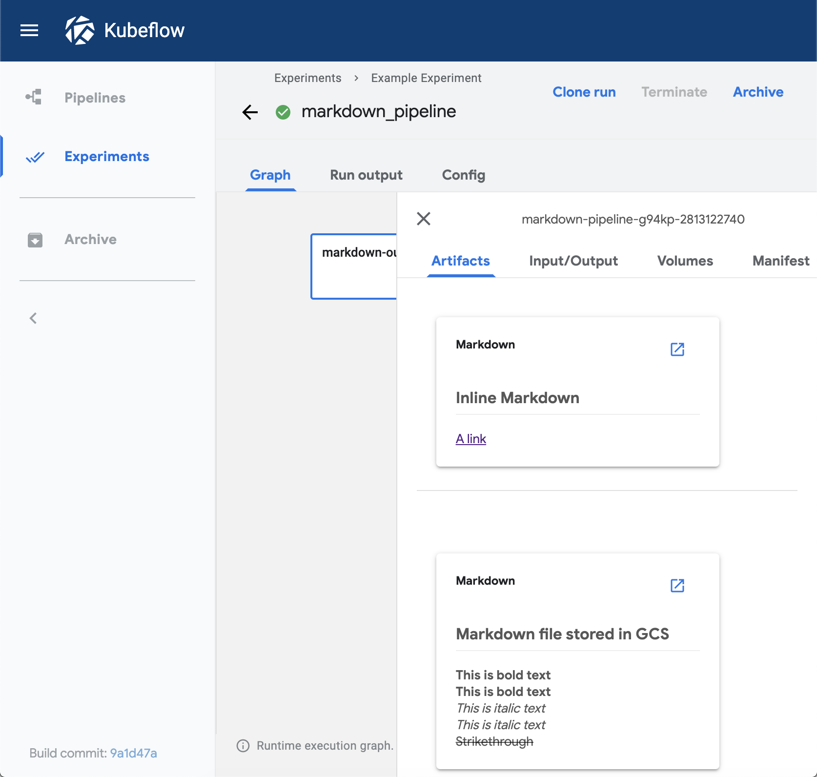
The markdown viewer renders Markdown strings on the Kubeflow Pipelines UI.
The viewer can read the Markdown data from the following locations:
- A Markdown-formatted string embedded in the
sourcefield. The value of thestoragefield must beinline. - Markdown code in a remote file, at a path specified in the
sourcefield. Thestoragefield can be empty or contain any value exceptinline.
Example:
def markdown_vis(mlpipeline_ui_metadata_path: kfp.components.OutputPath()):
  import json

  metadata = {
    'outputs' : [
    # Markdown that is hardcoded inline
    {
      'storage': 'inline',
      'source': '# Inline Markdown\n[A link](https://www.kubeflow.org/)',
      'type': 'markdown',
    },
    # Markdown that is read from a file
    {
      'source': 'gs://your_project/your_bucket/your_markdown_file',
      'type': 'markdown',
    }]
  }

  with open(mlpipeline_ui_metadata_path, 'w') as metadata_file:
    json.dump(metadata, metadata_file)
Visualization on the Kubeflow Pipelines UI:
ROC curve
Type: roc
Required metadata fields:
formatschemasource
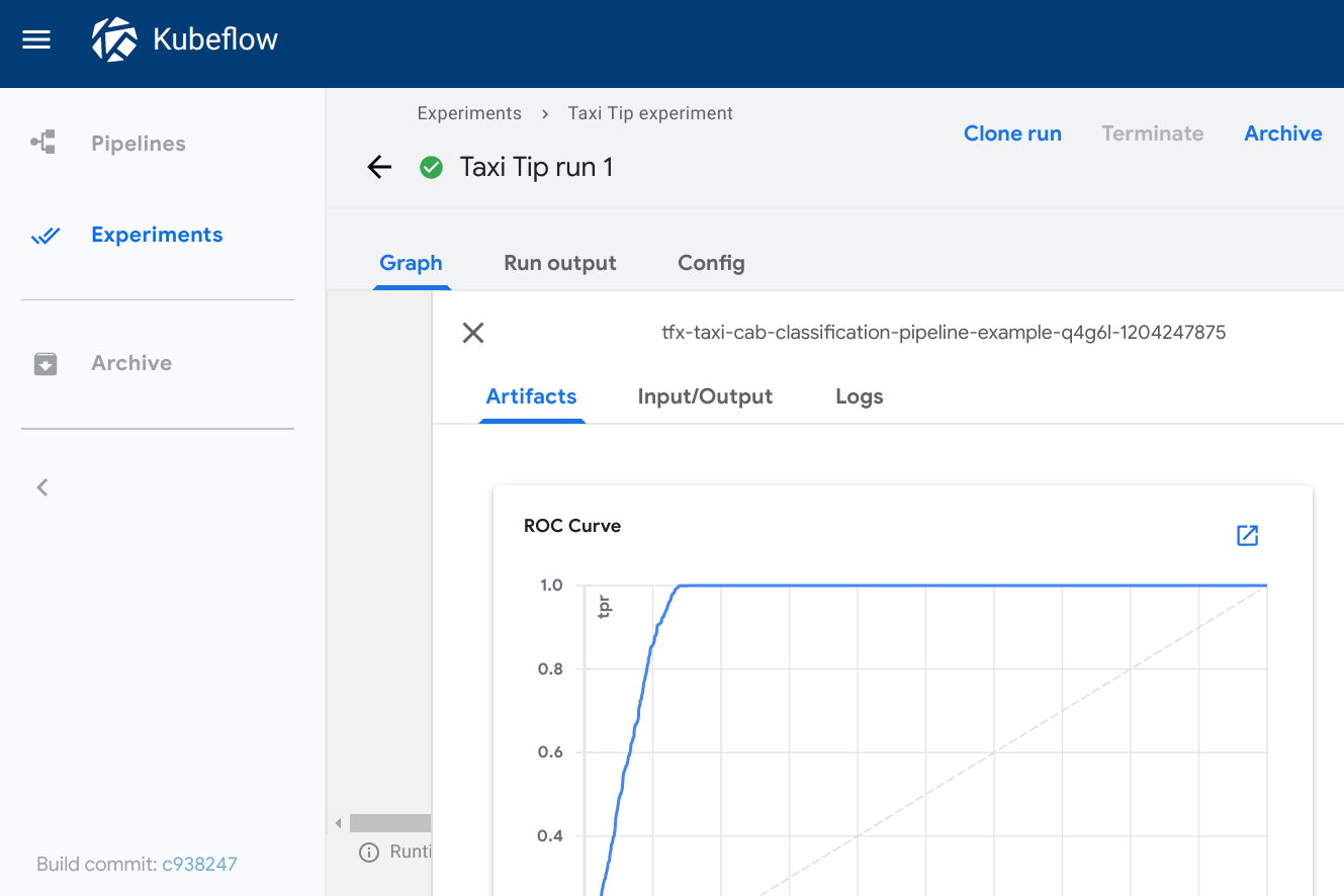
The roc viewer plots a receiver operating characteristic
(ROC)
curve using the data from the given source path. The Kubeflow Pipelines UI
assumes that the schema includes three columns with the following names:
fpr(false positive rate)tpr(true positive rate)thresholds
Optional metadata fields:
storage
When viewing the ROC curve, you can hover your cursor over the ROC curve to see
the threshold value used for the cursor’s closest fpr and tpr values.
Specify 'storage': 'inline' to embed raw content of the ROC
curve CSV file as a string in source field directly.
Example:
def roc_vis(roc_csv_file_path: str, mlpipeline_ui_metadata_path: kfp.components.OutputPath()):
  import json

  df_roc = pd.DataFrame({'fpr': fpr, 'tpr': tpr, 'thresholds': thresholds})
  roc_file = os.path.join(roc_csv_file_path, 'roc.csv')
  with file_io.FileIO(roc_file, 'w') as f:
    df_roc.to_csv(f, columns=['fpr', 'tpr', 'thresholds'], header=False, index=False)

  metadata = {
    'outputs': [{
      'type': 'roc',
      'format': 'csv',
      'schema': [
        {'name': 'fpr', 'type': 'NUMBER'},
        {'name': 'tpr', 'type': 'NUMBER'},
        {'name': 'thresholds', 'type': 'NUMBER'},
      ],
      'source': roc_file
    }]
  }

  with open(mlpipeline_ui_metadata_path, 'w') as metadata_file:
    json.dump(metadata, metadata_file)
Visualization on the Kubeflow Pipelines UI:
Table
Type: table
Required metadata fields:
formatheadersource
Optional metadata fields:
storage
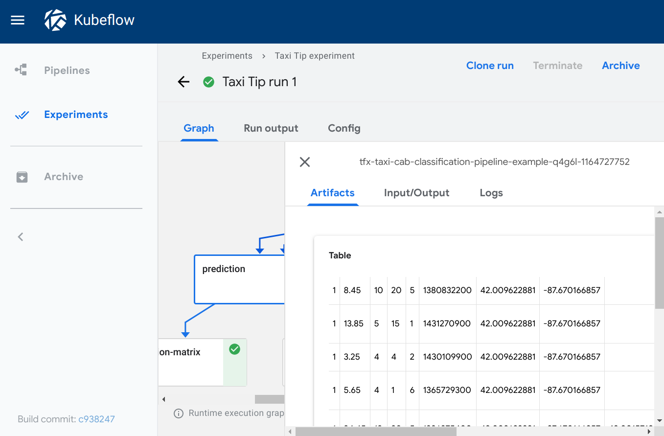
The table viewer builds an HTML table out of the data at the given source
path, where the header field specifies the values to be shown in the first row
of the table. The table supports pagination.
Specify 'storage': 'inline' to embed CSV table content string
in source field directly.
Example:
def table_vis(mlpipeline_ui_metadata_path: kfp.components.OutputPath()):
  import json

  metadata = {
    'outputs' : [{
      'type': 'table',
      'storage': 'gcs',
      'format': 'csv',
      'header': [x['name'] for x in schema],
      'source': prediction_results
    }]
  }

  with open(mlpipeline_ui_metadata_path, 'w') as metadata_file:
    json.dump(metadata, metadata_file)
Visualization on the Kubeflow Pipelines UI:
TensorBoard
Type: tensorboard
Required metadata Fields:
source
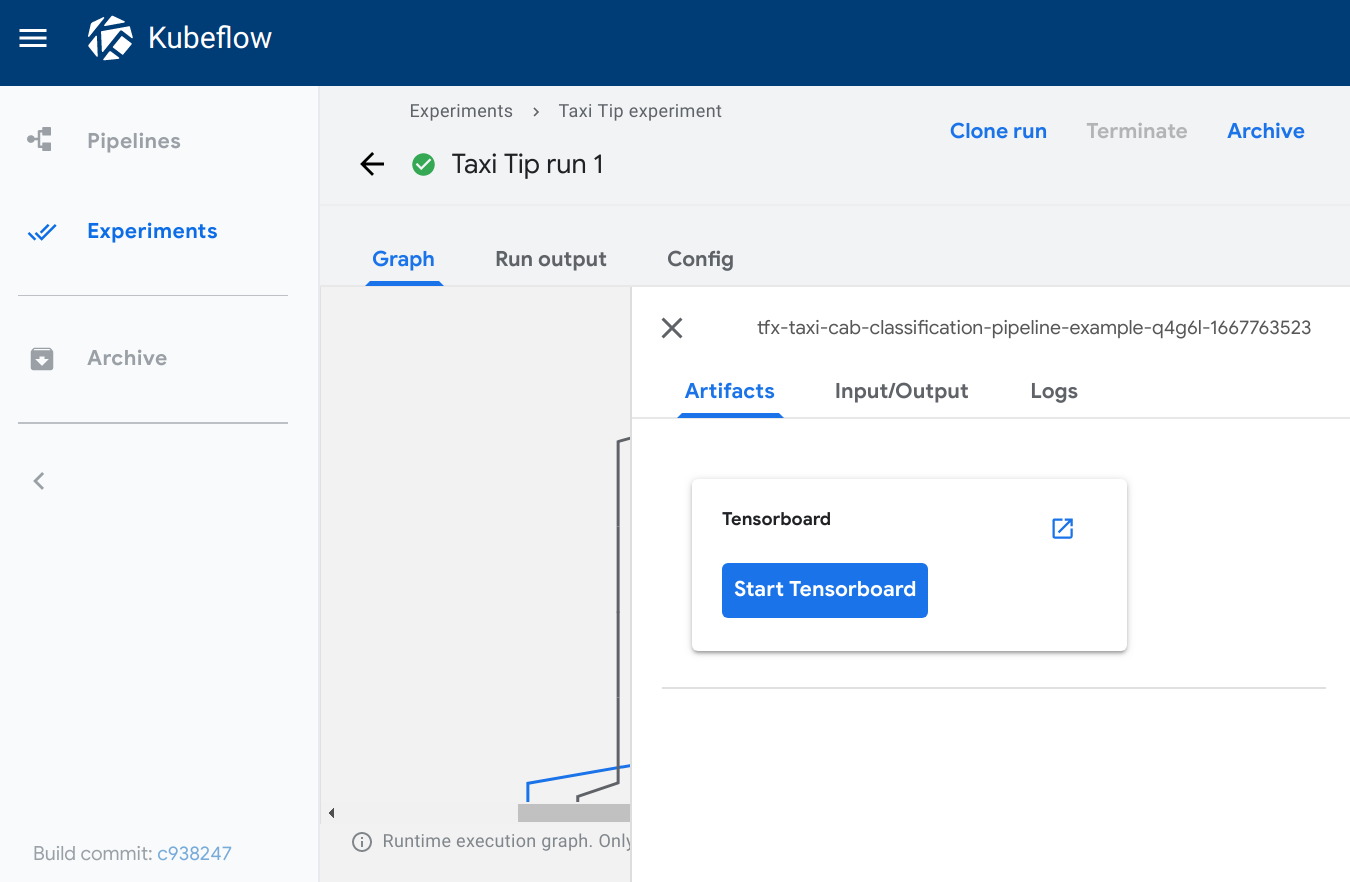
The tensorboard viewer adds a Start Tensorboard button to the output page.
When viewing the output page, you can:
- Click Start Tensorboard to start a TensorBoard Pod in your Kubeflow cluster. The button text switches to Open Tensorboard.
- Click Open Tensorboard to open the TensorBoard interface in a new tab,
pointing to the logdir data specified in the
sourcefield. - Click Delete Tensorboard to shutdown the Tensorboard instance.
Note: The Kubeflow Pipelines UI doesn’t fully manage your TensorBoard instances. The “Start Tensorboard” button is a convenience feature so that you don’t have to interrupt your workflow when looking at pipeline runs. You’re responsible for recycling or deleting the TensorBoard Pods using your Kubernetes management tools.
Example:
def tensorboard_vis(mlpipeline_ui_metadata_path: kfp.components.OutputPath()):
  import json

  metadata = {
    'outputs' : [{
      'type': 'tensorboard',
      'source': args.job_dir,
    }]
  }

  with open(mlpipeline_ui_metadata_path, 'w') as metadata_file:
    json.dump(metadata, metadata_file)
Visualization on the Kubeflow Pipelines UI:
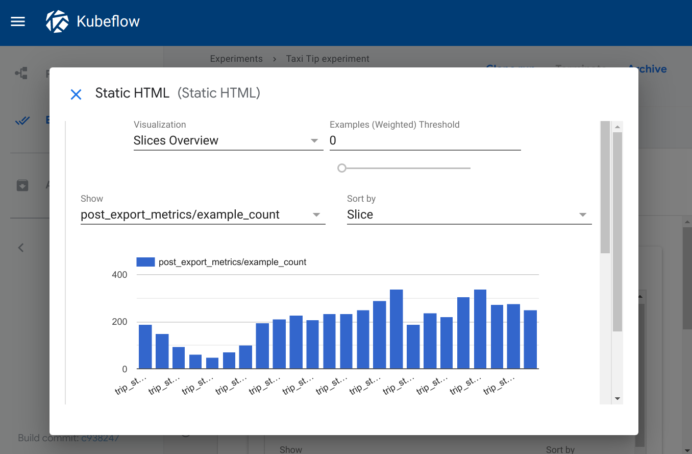
Web app
Type: web-app
Required metadata fields:
source
Optional metadata fields:
storage
The web-app viewer provides flexibility for rendering custom output. You can
specify an HTML file that your component creates, and the Kubeflow Pipelines UI
renders that HTML in the output page. The HTML file must be self-contained, with
no references to other files in the filesystem. The HTML file can contain
absolute references to files on the web. Content running inside the web app is
sandboxed in an iframe and cannot communicate with the Kubeflow Pipelines UI.
Specify 'storage': 'inline' to embed raw html in source field directly.
Example:
def tensorboard_vis(mlpipeline_ui_metadata_path: kfp.components.OutputPath()):
  import json

  static_html_path = os.path.join(output_dir, _OUTPUT_HTML_FILE)
  file_io.write_string_to_file(static_html_path, rendered_template)

  metadata = {
    'outputs' : [{
      'type': 'web-app',
      'storage': 'gcs',
      'source': static_html_path,
    }, {
      'type': 'web-app',
      'storage': 'inline',
      'source': '<h1>Hello, World!</h1>',
    }]
  }

  with open(mlpipeline_ui_metadata_path, 'w') as metadata_file:
    json.dump(metadata, metadata_file)
Visualization on the Kubeflow Pipelines UI:
Source of v1 examples
The v1 examples come from the tax tip prediction sample that is pre-installed when you deploy Kubeflow.
You can run the sample by selecting [Sample] ML - TFX - Taxi Tip Prediction Model Trainer from the Kubeflow Pipelines UI. For help getting started with the UI, follow the Kubeflow Pipelines quickstart.
The pipeline uses a number of prebuilt, reusable components, including:
- The Confusion Matrix
component
which writes out the data for the
confusion_matrixviewer. - The ROC
component
which writes out the data for the
rocviewer. - The dnntrainer
component
which writes out the data for the
tensorboardviewer. - The tfma
component
which writes out the data for the
web-appviewer.
Lightweight Python component Notebook example
For a complete example of lightweigh Python component, you can refer to the lightweight python component notebook example to learn more about declaring output visualizations.
YAML component example
You can also configure visualization in a component.yaml file. Refer to {name: MLPipeline UI Metadata} output in Create Tensorboard Visualization component.
Feedback
Was this page helpful?
Thank you for your feedback!
We're sorry this page wasn't helpful. If you have a moment, please share your feedback so we can improve.